Anisotropy Evaluation of a Femoral Head
This Bone Analysis tutorial provides step-by-step instructions for pre-processing a dataset of a femoral head, segmenting the bone, and computing vector field maps of anisotropy. Additional topics in this tutorial describe how to visualize and evaluate the generated vector fields.
Screen capture of completed tutorial

Before you start the tutorial, you should download and unzip the tutorial dataset — Femoral Head. This dataset, as well as the session file of the tutorial, is available on the ORS website at: http://www.theobjects.com/dragonfly/learn-sample-datasets.html.
The pre-processing steps required to prepare the dataset, which include aligning the dataset with the anatomical axes and cropping the derived dataset from the re-oriented view, are described in this section.
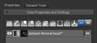
- Load the tutorial dataset or a similar sample, (see Importing Image Files).
The dataset appears in the Data Properties and Settings panel.
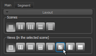
- Display the data in a 2x2 layout by clicking the Views icon, as shown below.
- Adjust window leveling, as required (see Window Leveling).
- In 3D views, it is often best to adjust window leveling on the histogram, as shown below.

- In 2D views, it is often quickest to use the Area
 tool to adjust leveling, as shown below.

- In 3D views, it is often best to adjust window leveling on the histogram, as shown below.
- Align the dataset with the anatomical axes, as follows:
- Select the 2D view showing the XY axis and then scroll to the slice that shows the full length of the bone.
- Click the Displace tool on the Move panel.

The Translate and Rotate tools appear in the selected view.
- Drag the Rotate tool, as shown below, to align the selected view with the anatomical axes.

NOTE You can use the Rotate and Translate tools in any MPR view of the dataset (see Translating and Rotating Objects).
- When you are satisfied with the result, click the Track tool to exit Move mode.
- Make sure the re-oriented view is selected and then right-click the dataset in the Data Properties and Settings panel.
- Choose Derive New from Current View in the pop-up menu.
The derived dataset appears in the Data Properties and Settings panel when the computation is complete.
- Crop the derived dataset, as follows:
- Display the derived dataset in a layout that includes multiple 2D views and/or a 3D view.
- Right-click the dataset in the Data Properties and Settings panel and then choose Crop in the pop-up menu.
The Dataset Cropper panel appears on the Dataset Tools tab on the right sidebar and a clip box appears in the views of the dataset.
- Do the following, as required:
- Adjust the clip box in the 2D views of the dataset, as shown below.

- Adjust the planes of the clip box in the 3D view of the dataset, as shown below.

- Adjust the clip box in the 2D views of the dataset, as shown below.
- Click the Apply button on the Dataset Cropper panel.

NOTE You can choose to apply cropping directly to the dataset or to create a new dataset.
- Continue to the next section to learn how the create the region of interest for analysis.


In this section, you will learn how to extract the required region of interest from a threshold range applied to the image data. Instructions for refining the initial segmentation are also included here.
- Display the cropped dataset in a multiple MPR layout, recommended.
See Scene Layouts and Views for information about changing layouts.
- Adjust window leveling, as required.
- Click the Segment tab on the left sidebar to access the ROI Tools panel.
The ROI Tools panel appears on the left sidebar.
- Do the following to create a region of interest with data values thresholded for mineralized bone:
- Make sure that the required dataset is selected in the Data Properties and Settings panel.
- Select the Define range option in the Range box on the ROI Tools panel.

- Drag the left or right Range sliders to change the minimum or maximum values of the intensity range or enter the required values in the Min and Max edit boxes.
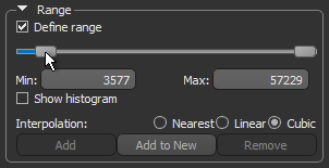
- Verify the selected range on other images in the image stack and other views of the dataset, recommended.

- Click the Add to New button to create a region of interest in which all voxels within the selected range are labeled.

A new region of interest is added to the Data Properties and Settings panel. Information about the new ROI is displayed in the lower section of the panel (see ROI Properties and Settings).
- Uncheck the Define range option in the Range box.
- Remove noise and other unwanted objects from the region of interest as follows:
- Right-click the region of interest in the Data Properties and Settings panel and then choose Process Islands > Isolate (6-connected) nth First Biggest in the pop-up menu.
- Enter 1 in the Isolate Biggest Count dialog and then click the OK button.
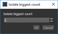
All unconnected objects that are smaller than the largest object in the region of interest are removed from the ROI (see Processing Islands).
NOTE With this initial bone segmentation you can separate the cortical shell from the trabecular interior automatically and then compute morphometric indices (see Computing Cortical and Trabecular Measurements). Other options include creating a graph for topological analysis (see Creating Sparse and Dense Graphs), exporting the ROI as a binary image (see ROI as Binary), closing holes for 3D print preparation (see Fill Connected Pores with a Diameter Smaller Than), and creating a distance map for other analysis purposed (see Creating Distance Maps).
- Continue to the next section to learn how to compute vector field-based maps of anisotropy.

This section provides step-by-step instructions for computing a 3D vector field-based map of anisotropy.
- Make sure that the required region of interest is selected in Data Properties and Settings panel.
- Create a box that either entirely or partially encloses the region of interest as follows:
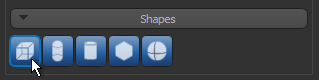
- Click the Box button in the Shapes panel.
A new Box shape appears in the Data Properties and Settings panel. Click the Eye icon to show the box in the workspace views.

- Adjust the box in the 2D and/or 3D view of the region of interest, as required.
You can resize and rotate the box, as well as change its position within a 2D or 3D view with the control points (see Editing Shapes).

NOTE Large box sizes and small spacing and/or radius of influence settings will increase computation time.
- Click the Box button in the Shapes panel.
- Choose Tools > Bone Analysis on the menu bar to open the Bone Analysis dialog.
- Do the following on the Mappings tab:
- Choose Surface normals in the Algorithm drop-down menu.
- Choose the region of interest that you created for this tutorial in the Bone segmentation drop-down menu.

- Choose the box that encloses the area that you want to include in your analysis in the Area box drop-down menu.

- Enter a value of 0.002 m in the Spacing edit box.
NOTE Although the highest resolution, or lowest spacing, is 0.085 mm, this is increased to reduce processing times as the entire 3D shape of the femoral head will be mapped.
- Select a value between 1 and 3 mm in the Radius of influence edit box.
NOTE The radius of influence defines the kernel size, or elementary volume, within which anisotropy will be evaluated. You should note that a too small radius of influence may result in a low signal-to-noise ratio, while a too high radius can result in averaging and edge effects.
- Choose Projection-based in the Anisotropy drop-down menu.

- Choose a number of iterations in the Mesh smoothing (repetitions) spin box, optional.
- Click the Compute Mapping button.

This will map the anisotropy of 3D surfaces — their preferred orientation between 0 (random) and 1 (perfectly aligned) and the direction of that preferred orientation with respect to the Cartesian coordinates.
Two new items — a vector field and scalar-based anisotropy dataset — appear in the Data Properties and Settings panel after all computations are complete.

- Continue to the next section to learn how to examine and evaluate the computed vector field-based map.

This section describes the different settings that can be applied to the vector field-based anisotropy map that was computed in this tutorial.
In the examples below, the top row corresponds to the anterior view, while the bottom row provides views of the posterior aspect. The images on the top left shows the relationship between the box and the 3D rendering of the femoral head at the default settings. The images in the middle show anisotropy mapped by magnitude, with red being very anisotropic and blue very isotropic. The images on the right show the same maps replotted in such a way that the color corresponds to the vector orientation. This is case, red is along the X axis, green is along the Y axis, and blue is along the Z axis.
Vector field-based maps of anisotropy

The properties and settings for the 3D vector field appear in the bottom section of the Data Properties and Settings panel.
- Maximize the 3D view in the workspace, recommended.
- You can maximize a view by double-clicking it or you can right-click and then choose Maximize View in the pop-up menu.
- Select the 3D vector map you created and make it visible in the 3D view.
- To make an object visible in a 3D view, click the Eye icon in the Data Properties and Settings panel.
The 3D vector field-based anisotropy map appears in the 3D view at the default settings, with the vectors corresponding to the highest surface anisotropy colored yellow and those corresponding to the lowest , or isotropy, colored blue..

Information and settings related to the 3D vector fields appear in the bottom section of the Data Properties and Settings panel.
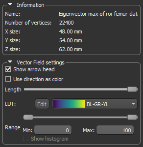
NOTE In most cases, you should hide the rendering of the dataset if it is visible in the 3D view.
- To make an object visible in a 3D view, click the Eye icon in the Data Properties and Settings panel.
- Change the settings applied to the 3D vector field-based map, as described below.
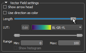
- Uncheck the Show arrow head option. This usually improves the visibility of the vectors in the field.
- Use the Length slider to adjust the length of vectors, optional.
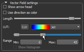
- Choose another look-up table (LUT) in the LUT drop-down menu.

NOTE The Jet LUT is often a good color scheme choice. In this LUT, vectors corresponding to the highest surface anisotropy are colored red, while those corresponding to the lowest, or are isotropic, are colored blue.

- Threshold the vector field-based map to show only high or low anisotropy areas with the Range slider, as shown below, optional.
- Check the Use direction as color option.
Checking this option will re-code the vector map in accordance with the orientation of the vectors — red for the X axis, green for the Y axis, and blue for the Z axis.

- Compute high-resolution maps in different orientations and compute volume fractions, optional.
These options are described in the tutorial Anisotropy and Volume Fraction Mapping of a Proximal Femur.